Get a Custom Essay Paper that meets your expectations by clicking ORDER
Lab Report
Students are required to write a laboratory report, not exceeding 1,500 words in accordance with APA (American Psychological Association, 6th edition) formatting requirements.
The report is based on the experiment conducted in laboratory classes during Week 3 of the semester. The report should include:
A literature review and critique of the relevant literature.
What is Mindfulness?- a paper trying to operationalise Mindfulness
Selective Attention IMPROVES under stress- this paper argues that being stressed can improve attention performance
Selective Attention is IMPAIRED by stress- this paper argues that stress impairs selective attention (although using a different task to us to measure attention BUT a similar method of inducing stress)
Get a Custom Essay Paper that meets your expectations by clicking ORDER
Want help to write your Essay or Assignments? Click here
Mapping DNA using restriction Enzymes and electrophoresis
Mary Smith
Chem I – Sect C
10/12/20XX
Sediment in Water – Lab #3
Koeck (Edit this part with your details)
Abstract
This laboratory report describes the experiment that was conducted using the restriction enzymes- restriction endonuclease- to manipulate the DNA molecules. The restriction enzyme has the capacity to recognize DNA sequences, and cleaving the DNA at that specific site. The endonuclease was used in conjunction with electrophoresis to map 2, 686 base pair of the pUC 19 plasmid. The plasmid cut into fragments, was separated using gel electrophoresis based on the charge and size.
Introduction
The first stage of DNA analysis for refined DNA such as gene expression and DNA sequencing is the construction of the DNA map. This has been done previously by scientists who used enzymes that are naturally occurring often referred to as restriction enzymes, to cut the large pieces of large molecule of DNA into small pieces. The fragments are then separated and sorted through the use of gel electrophoresis and the results obtained, they can be used to reconstruct the map of DNA molecule. This process is commonly referred to as mapping (Hughes and Moody, 2007).
This experiment was conducted using the restriction enzymes- restriction endonuclease- to manipulate the DNA molecules. The enzyme has the capacity to recognize specific DNA sequences, and cleaving the DNA at that specific site. The endonuclease will be used in conjunction with electrophoresis, which will be used to map 2, 686 base pair of the pUC 19 plasmid. The plasmid will be cut into fragments, which will be separated using gel electrophoresis based on the charge and size.
Want help to write your Essay or Assignments? Click here
Experiments (materials and methods)
Materials
Gel electrophoresis apparatus; Gel plates, comb to make wells, chamber cover, and chamber electrophoresis. Power supply with electrodes, deionized water, hot plate/ microwave, agarose, 250-Ml Erlenmeyer flask, and 100 ml graduated cylinder, pUC 19 plasmid DNA, restriction buffers, ice, restriction enzymes, molecular weight markers (lambda DNA), Ava II, Pvu II, gel loading dye (bromophenol blue), 15 1.5 Eppendorf’s, thermometer and metric rulers. Other common materials include, container that contains TBE solution, water bath (37 C), Floating rack, 60º C hot plate, cooler containing crushed ice, Polaroid camera with 667 Polaroid film, methylene blue stain, UV protective equipment, distilled water and non-frost free freezer.
Method
To make the Gel electrophoresis field, 1.0% of agarose was prepared as follows. To make 100 ml of gel, 1.0 g of the agarose was weighed and placed into the 250 ml glass beaker. 100 ML OF 1x TBE (Tris-Borate-EDTA) buffer was added. The mixture was heated in the hot pan for 30 seconds, shaking gently until all the agarose had melted completely. The solution was cooled and stored in a refrigerator.
The second day, pan was filled with water and was adjusted to 60 º C. The agarose was poured as follows; the agarose bottle that had been stored in day 1 was melted in the hot water bath. Firmly, the ends of the gel tray were sealed using a labelling tape, and a comb was placed on the slots, near the end of the tray, approximately, 40 ml of the agarose was poured in each of the tray, and was let cool for 15 minute to solidify.
During enzyme restriction stage, all enzymes and DNA aliquots were kept in ice. The four microtubes and reagents were labelled and stored as indicated below
Reagents
Ava II
Pvu II
Control
10 x Buffer
4 µl
4 µl
4 µl
DNA
4 µl
4 µl
4 µl
PvuII
0 µl
2 µl
0 µl
Ava II
2 µl
0 µl
0 µl
Water
30 µl
30 µl
30 µl
The micropipette was set to collect 4µl and 4 10X restriction buffer to each of the tube. The similar process was followed to load 4.0 µl of DNA, but using a different tube, to the control tube, 32 µl of distilled water was added whereas in the other reaction tube, 30 µl of distilled water was added.
The microtubes caps were closed and were heated in the 55 ºC for 10 minutes and were placed immediately on ice for 2 minutes. 2 µl of the appropriate restriction enzymes were added as shown in the grid above. The microtubes caps were closed, tapped the tube gently to bring all the liquid to the bottom, and were incubated overnight at 37 C.
Want help to write your Essay or Assignments? Click here
To run the electrophoresis, the tubes were collected and placed in the ice tubes and the gel electrophoresis field was set up. The microtubes were heated in 60º C water bath for 3 minutes. 4 µl of the loading dye was added in each of the reaction tube. 20 µl of each sample was loaded in the well, and the current was turned on for 30 to 45 minutes. The gel was stained using the methylene blue solution in 0.1 TBE and was stained for 2 hours at room temperature. Observations were made and photograph was taken.
Results
There were several errors that we done during the preparation of the gel electrophoresis field. The first preparation did not gel, and the mistake could not be traced. This led to preparation of the second gel, which eventually worked perfectly. The loading of the DNA was also somewhat troublesome due to shaking of the hands, but I managed to pull it off, with the assistance of laboratory technician and my peers.
The following observations was made
1=2-log DNA (0.1-10 kb) molecular weight marker
2=pUC19 digested with AvaII, at 2464bp and 222bp
2 cuts =pUC19 digested with PvuII at 2364bp and 332 bp
4 cuts =pUC19 digested with AvaII and PvuII at 2464 bp, 2364bp, 332 bp and 222bp.
The control field had no fragments. Thebase pair at which the cuts occurred is almost the same number as those predicted by the pUC 19 maps.
Want help to write your Essay or Assignments? Click here
Discussion
The pCU19is a 26866 base pairs, and thus its kb can be estimated to be 2.7 kb. It is small, and a high copy number in E.coli plasmid, which contain pBR322 and M13MP19. It has multiple cloning sites, where each unique enzyme can cause restriction, thus facilitating the recombinant technology (Omoto and Lurquin, 2004).
The microtubes containing DNA were heated ath 60C to break hydrogen bonds at the end of the linear DNA. Addition of the dye also stopped the restriction reaction from taking place. After running the gel electrophoresis, DNA being negatively charged, it migrated towards the cathode, inform of bands of specific size. The controls had no fragments because the DNA was not digested by any restriction enzyme (Twyman, 2009).
The following observations were made; there were two cuts when pUC19 was digested with AvaII, at 2464bp and 222bp. This was also the same when pUC19 digested with PvuII, and the cuts were estimated to be at 2364bp and 332 bp. In double cleavage, a total of 4 cuts were observed when pUC19 was digested with AvaII and PvuII at 23640 bp, 2464 bp, 322 bp and 222 bp.
The control field had no fragments. The cuts are almost the same base pair number as those predicted by the pUC 19 maps. However, when compared the results from the attached pUC 19 map, the AvaII points should be digested at 1837 bp and 2059 bp, whereas, PvuII at 306 bp and 628 bp. The minor deviations could be associated with accuracy of recording the base pairs. The 4 cuts obtained by the double digests indicate that restriction enzymes recognize DNA sequences and cut them at that site (Twyman, 2009).
Want help to write your Essay or Assignments? Click here
Conclusion
The study objectives were achieved, restriction activity took place. This technique is a very important technique as it helps on interacts with the basics of cloning techniques and tools used in molecular biology.
References
Hughes, S. and Moody, A. (2007). PCR. Bloxham: Scion.
Omoto, C. and Lurquin, P. (2004). Genes and DNA. New York: Columbia University Press.
Want help to write your Essay or Assignments? Click here
Tensile Testing
Summary
Tensile testing is undeniably the most imperative experimental method that is used in determining the characteristics or properties of various materials for the purpose of predicting their behaviours as well as how they would respond to tension in their real world engineering applications. The specific properties of material that are determined through tensile test include maximum elongation, ultimate tensile strength as well as reduction in area.
The material properties are imperative in the selection of materials for mechanical design. In this lab experiment, a tensile tester was used to determine tensile properties of specimens of three materials namely duralumin, PVC and aluminium.
From the obtained tensile test results, duralumin properties including tensile strength (N/m2), yield stress (N/m2) and % elongation were 0.054 N/m2, 1.29231 N/m2 and 29.23 % respectively. In addition, those of PVC were 0.928 N/m2, 37.73585 N/m2 and 37.74 % for tensile strength (N/m2), yield stress (N/m2) and % elongation respectively; whereas those of aluminium were 0.083 N/m2, 0.65789 N/m2 and 65.79 % for tensile strength (N/m2), yield stress (N/m2) and % elongation respectively.
These properties show that both duralumin and aluminium are ductile and tough compared to PVC which indicate stiffness properties. These properties are further illustrated in the stress-strain plots of each material. In conclusion, the tensile test results obtained from this lab experiment are useful in determining tensile properties of materials as well as providing valuable information concerning not only the material’s mechanical behaviours but also its engineering performance.
Want help to write your Essay or Assignments? Click here
Introduction
The determination of the mechanical properties or characteristics of materials is done by performing laboratory experiments that are carefully designed so that they can be replicated under the same service conditions as nearly as possible. In real world applications of materials in mechanical engineering, there is involvement of myriad of factors in the determination of the nature in which application of loads can be done on a material (Czichos, 2006).
According to Ashby (2006) tensile testing is a fundamental test in material science where controlled tension is subjected to a sample until failure, and the obtained results often used for quality control and selection of materials for application. According to Hibbeler (2004), the specific properties of material that are determined through tensile test include maximum elongation, ultimate tensile strength as well as reduction in area. The material properties are imperative in the selection of materials for mechanical design (Davis, 2004).
Tensile testing is without any doubt the experimental method that is used in determining the characteristics of various mechanical materials with an intention of predicting the behaviours of such materials and how they would respond to tension in their real world engineering applications (Czichos, 2006).
The main objective of this experiment is to conduct an experimental tensile testing on various mechanical materials, i.e. duralumin, aluminium and PVC in order to determine and compare their characteristics, which can be used to predict their particular behaviours in real world engineering applications. The other main objective is to plot graphs describing the characteristics or properties of these materials as obtained in the tensile testing results.
As a result, graphs depicting the properties of these materials shall be plotted by stretching the samples of each of provided materials of known dimensions to destruction upon applying force subsequent to noting the ensuing elongation.
Thus, tensile test results obtained in this lab has many benefits because they enable a stress-strain diagram to be obtained, which is useful in determining the tensile properties of materials as well as providing valuable information concerning not only the material’s mechanical behaviours but also its engineering performance (Hibbeler, 2004).
Want help to write your Essay or Assignments? Click here
Theory
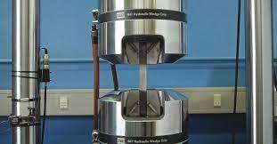
The topic covered in this lab experiment is focused to testing of tensile properties of various materials that have different compositions. Figure 1 illustrated below shows a machine used in tensile testing that resembles the one used during the laboratory experiment session. Tensile test is a destructive in nature, in which an axial is subjected to a sample of the material to be tested, and the specimen has to be of a standard shape as well as dimensions.
During a typical procedure for a tensile testing laboratory experiment, a specimen that dog-bone shaped is usually gripped at the top and bottom of the tensile machine on its two ends prior to pulling so that elongation occurs at a determined rate that is controlled up to its breakpoint (Hibbeler, 2004). Tensile testers vary mainly on the basis of pulling rate and maximum load, and their setup during an experiment could be varied for the purpose of mechanical testing of different materials through tensile test (Czichos, 2006).
Figure 1: Tensile test 1 (A photograph of a tensile machine)
For analytical purposes, stress (σ) vs. strain (ε) is plotted from a tensile test experiment results, and this can be done either manually or automatically (Czichos, 2006). In the metric system, the usual measure for stress is Pa or N/m2, such that 1 Pa = 1 N/m2. From the laboratory experiment, the calculation of stress values is done through division applied force (F) by the cross-sectional area (A) of the machine, which is measured before the experiment is run (Hibbeler, 2004). Equation 1 and 2 below are used to calculate stress and strain values respectively.
Want help to write your Essay or Assignments? Click here
A typical stress-strain plot would look like figure 2 below, which is an example of a generalised and typical representation of a stress-strain curve for ductile metal materials (Davis, 2004). Figure 2 below indicates that the curve has four parts: elastic region, yielding region, strain hardening region and necking region, which occur in almost all materials except the strain hardening region commonly occurring in metallic materials (Czichos, 2006).
In theory, even without the specimen’s cross-sectional area measurement during the tensile testing lab experiment, it is possible to construct a “true” stress-strain curve based on the assumption that there is constant amount of the material. Using this concept, it is possible to calculate both the true strain (εT) and the true stress (σT) using Equation 3 and Equation 4, respectively.
Want help to write your Essay or Assignments? Click here
In the curve shown in Figure 2 above, the linear region, which is known as the elastic region depicts the region of the curve where the behaviour of the material is elastic. Equation 5 can be used to calculate the slope of the curve, which is an intrinsic property and is a constant of a material referred to as the elastic modulus (E). Its SI unit is Pascal (Pa).
Figure 3 shown below illustrates a typical stress-strain curve plot, and it shows that different materials, both metals and polymers portray varied properties under tension, which determines their greatest extent of deformation or ductility before fracture whereby some have very steep or relatively gentle elastic moduli.
According to Hibbeler (2004), mechanical properties of both metals and polymers are generally dependent on their molecular weights, extent of crystallinity, as well as glass transition temperature, Tg. For instance, if materials under consideration are highly crystalline and with a Tg higher than room temperature usually tend to be brittle, and vice versa (Davis, 2004).
On the other hand, when semi-crystalline polymers or materials are subjected to tensile testing, there will be an alignment of the amorphous chains usually evident for translucent and transparent materials, which have a tendency of becoming opaque after they turn crystalline.
The stress-strain curve is used to give Young’s Modulus based on the run and rise of the slope, which is calculated similar to the gradient of a curve within the yield strength range prior to the material entering the ultimate strength phase subsequent to fracturing (Ashby, 2006)
Figure 3: A typical stress-strain curve plot
Equipment and Procedure
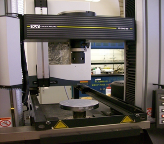
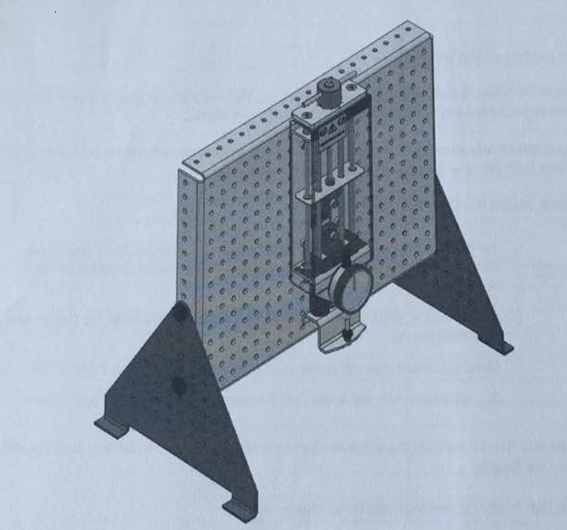
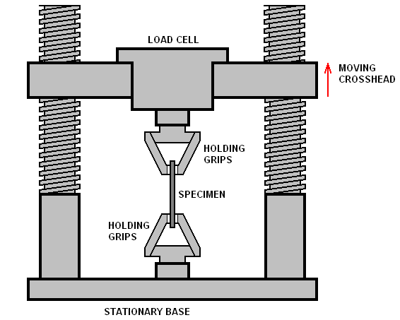
Prior to beginning the experiment, the supplied guidance notes were carefully read after which the experiment setup of the tensile testing machine was confirmed to be alright. A photograph of the experiment is shown in Figure 4 below. Consequently, Figure 5 that follows is a detailed schematic diagram of a tensile testing machine showing the main parts.
Holding grips are used both at the top and bottom to hold the specimen in place firmly; load cell is used to provide the required weight depending on the sample material’s load range and sensitivity. In addition, the stationary base is used to ensure stability of the machine, while moving crosshead is used to adjust the load cell subjected to the material.
Figure 4: Experiment SetupPhotograph of a Tensile Testing Machine
Figure 5: Detailed Schematic of a Tensile Testing Machine
Prior to starting the tensile test the safety guard was fitted followed by the selection of the specimen, which was then followed by the use of Dial Calliper for the width and thickness measurement of the specimen at gauge length as well as the cross-sectional area was determined.
The initial length of the specimen was measured and recorded or reference. The specimen was then fitted to the Tensile Tester followed by setting to zero the Dial Indicator, and the readings obtained for each specimen on the Vertical Scale were noted. Then the Load Nut was turned clockwise gradually in steps of 0.2 mm up to the length of 5 mm in a serial manner, and then followed by larger steps of 1 mm and 10 mm until the specimen broke.
The applied rate was kept consistent, i.e. 5 seconds were taken between each 0.2 mm of Load Nut turning followed by another 5 seconds for the readings to be recorded. The Dial Indicator value was recorded at each step, and for PVC specimen, this was done immediately after the load was change in order to obtain consistent results.
Want help to write your Essay or Assignments? Click here
The specimen elongation was checked by removing the specimen from the tensile tester and the broken ends were pushed together in order to measure the final length. The next step was conversion of the readings of the Dial Indicator into force values. The extension of the specimens at each step was determined by subtracting the readings of the Dial Indicator from those of the Load Nut movement.
The obtained values of force and extension were consequently converted to stress as well as nominal strain values, which were subsequently plotted on the chart paper for each specimen, i.e. the steel, PVC and alloy. The yield points and tensile strengths for each specimen were noted from the charts. Finally, the elastic region gradients for each specimen were determined for subsequent comparison of the stiffness of the materials.
Results and Discussion
The tensile testing results are shown in table 1 below where the results of the three specimens are illustrated on properties such as force, extension, strain and stress. In addition, tensile strength, yield stress and percentage of elongation are calculated and included in the table for duralumin, PVC and aluminium respectively. Furthermore, the stress-strain curves for each of the specimens are plotted to illustrate the relationships between the two properties in Figures 6, 7 and 8.
Table 1: Data collected from experiment 1
Duralumin
PVC
Aluminium
Load Nut movement (mm)
Dial Indicator (mm)
Force (N)
Extension (mm)
Stress σ N/m2
Nominal Strain ԑ
Load Nut movement (mm)
Dial Indicator (mm)
Force (N)
Extension (mm)
Stress σ N/m2
Nominal Strain ԑ
Load Nut movement (mm)
Dial Indicator (mm)
Force (N)
Extension (mm)
Stress σ N/m2
Nominal Strain ԑ
0
0
0
0
0
0
0
0
0
0
0
0
0
0
0
0
0
0
0.2
1.65
0.2
-1.45
0.12121
-0.8787
0.2
0.36
0.2
-0.16
0.55556
-0.44444
0.2
0.62
0.2
-0.42
0.32258
-0.67742
0.4
1.865
0.4
-1.465
0.21448
-0.7855
0.4
0.495
0.4
-0.095
0.80808
-0.19192
0.4
0.98
0.4
-0.58
0.40816
-0.59184
0.6
1.91
0.6
-1.31
0.31414
-0.6858
0.6
0.52
0.6
0.08
1.15385
0.15385
0.6
1.29
0.6
-0.69
0.46512
-0.53488
0.8
1.96
0.8
-1.16
0.40816
-0.5918
0.8
0.63
0.8
0.17
1.26984
0.26984
0.8
1.41
0.8
-0.61
0.56738
-0.43262
1
2.09
1
-1.09
0.47847
-0.5215
1
0.61
1
0.61
1.63934
1
1
1.52
1
-0.52
0.65789
-1
1.2
2.14
1.2
-0.94
0.56075
-0.4392
1.2
0.59
1.2
0.61
2.0339
1.0339
1.2
1.4
2.28
1.4
-0.88
0.61404
-0.3859
1.4
0.58
1.4
0.82
2.41379
1.41379
1.4
1.6
2.44
1.6
-0.84
0.65574
-0.3442
1.6
0.56
1.6
1.04
2.85714
1.85714
1.6
1.8
2.55
1.8
-0.75
0.70588
-0.2941
1.8
0.56
1.8
1.24
3.21429
2.21429
1.8
2
2.68
2
-0.68
0.74627
-0.2537
2
0.55
2
1.45
3.63636
2.63636
2
2.2
2.81
2.2
-0.61
0.78292
-0.2170
2.2
0.53
2.2
1.67
4.1509
3.15094
2.2
2.4
2.89
2.4
-0.49
0.8304
-0.1695
2.4
0.53
2.4
1.87
4.5283
3.5283
2.4
2.6
2.92
2.6
-0.32
0.8904
-0.109
2.6
0.52
2.6
2.08
5
4
2.6
2.8
2.98
2.8
-0.18
0.9396
-0.060
2.8
0.51
2.8
2.29
5.4902
4.4902
2.8
3
3.1
3
0.1
0.9677
0.0322
3
0.5
3
2.5
6
5
3
3.2
3.11
3.2
0.09
1.0289
0.0289
3.2
0.5
3.2
2.7
6.4
5.4
3.2
3.4
3.16
3.4
0.24
1.0759
0.0759
3.4
0.49
3.4
2.91
6.9387
5.93878
3.4
3.6
3.19
3.6
0.41
1.1285
0.1285
3.6
0.49
3.6
3.11
7.3469
6.34694
3.6
3.8
3.22
3.8
0.58
1.1801
0.1801
3.8
0.48
3.8
3.32
7.9166
6.91667
3.8
4
3.23
4
0.77
1.2383
0.2383
4
0.47
4
3.53
8.5106
7.51064
4
4.2
3.25
4.2
0.95
1.2923
0.2923
4.2
0.46
4.2
3.74
9.1304
8.13043
4.2
4.4
4.4
0.46
4.4
3.94
9.5652
8.56522
4.4
4.6
4.6
0.45
4.6
4.555
10.222
10.12222
4.6
4.8
4.8
0.41
4.8
4.39
11.707
10.70732
4.8
5
5
0.36
5
4.64
13.888
12.88889
5
6
6
0.33
6
5.67
18.181
17.18182
6
7
7
0.29
7
6.71
24.13
23.13793
7
8
8
0.29
8
7.71
27.586
26.58621
8
9
9
0.28
9
8.72
32.142
31.14286
9
10
10
0.265
10
9.735
37.73
36.73585
10
Tensile Strength (N/m2): 0.054 N/m2
Tensile Strength (N/m2):0.928 N/m2
Tensile Strength (N/m2): 0.083 N/m2
Yield Stress (N/m2): 1.29231 N/m2
Yield Stress (N/m2): 37.73585 N/m2
Yield Stress (N/m2): 0.65789 N/m2
% Elongation: 29.23%
% Elongation: 37.74%
% Elongation: 65.79%
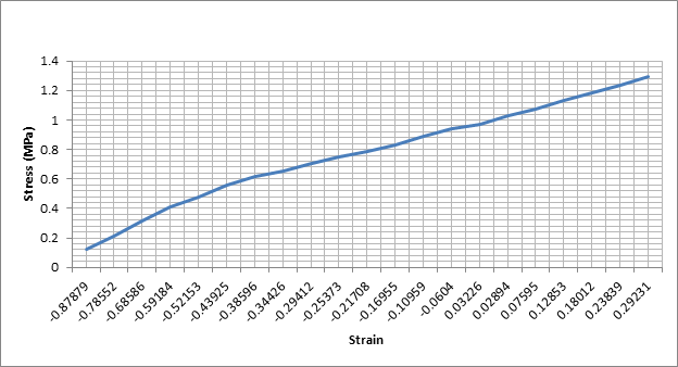
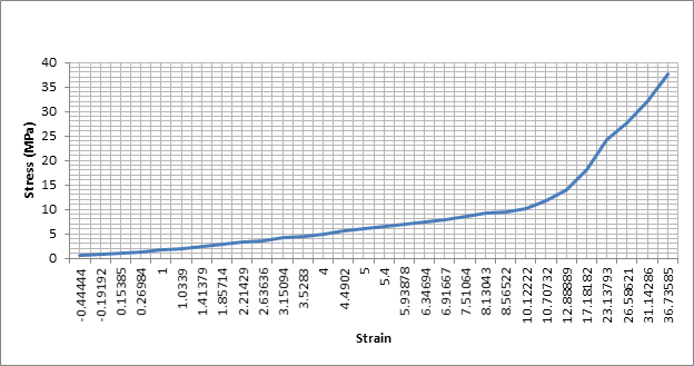
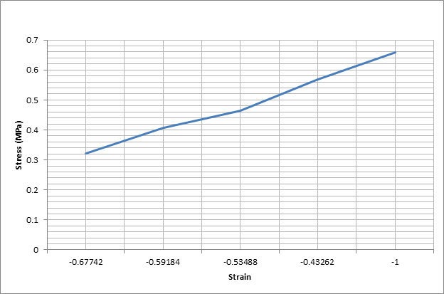
The figures below show the stress-strain plots for each of the specimens tested;
Figure 6: Duralumin Stress-strain plot
Figure 7: PVC Stress-strain plot
Figure 8: Aluminium stress-strain plot
From the tensile test results shown in table 1 above, duralumin properties including tensile strength (N/m2), yield stress (N/m2) and % elongation were 0.054 N/m2, 1.29231 N/m2 and 29.23 % respectively. In addition, those of PVC were 0.928 N/m2, 37.73585 N/m2 and 37.74 % for tensile strength (N/m2), yield stress (N/m2) and % elongation respectively; whereas those of aluminium were 0.083 N/m2, 0.65789 N/m2 and 65.79 % for tensile strength (N/m2), yield stress (N/m2) and % elongation respectively.
These characteristics show that both duralumin and aluminium are ductile and tough compared to PVC which indicate stiffness properties. These properties are further illustrated in the graphs.
Two specimen of the materials, i.e. duralumin and aluminium produced gradients that are relatively the same in their elastic region mainly because they are both metals even though one is a pure metal while the other one is an alloy. The reason why there is a significant difference between tensile properties of the two materials and PVC (which is a polythene polymer) is that, the chemical compositions are totally different hence making them to behave differently under tension (Davis, 2004).
Constant temperature and force application rate are very important for PVC specimens because it is composed of polymers, which easily change even with slight variations of temperature or force and this makes it imperative to ensure that both temperature and force application rate are maintained constant in order to obtain consistent results (Czichos, 2006).
Want help to write your Essay or Assignments? Click here
Some of the important shortcomings of the experimental apparatus is that, when large forces are been exerted there is a likelihood of the equipment to flex resulting to some extent of displacement (Tarr, n.d.). This machine’s displacement is often mistakenly read and recorded as a displacement of the specimen, and can lead to false results. To address this challenge, the tensile machine should be firmly held on the bench to ensure that no flexing occurs when large forces are applied on the specimens (Ashby, 2006).
Conclusion and Recommendations
By undertaking this lab experiment, I have learned a lot about the concept of tensile testing and my understanding on the same has significantly improved. For instance, I have gained more insights on how tensile properties differ between materials based on their chemical composition. In particular, the tensile properties of the three materials including tensile strength (N/m2), yield stress (N/m2) and % elongation varied considerably, especially between PVC and the other two materials (duralumin and aluminium) mainly due to their composition differences.
The specific aspects of the procedure of this lab experiment that contributed immensely to my learning was about the extension or elongation variations observed between materials before they broke, whereby significant difference was observed between metal specimens and PVC specimens. Prior to doing the lab experiment I had difficulties in comprehending how the tensile testing concept is used in choosing materials for mechanical engineering applications.
However, after the lab experiment my difficulties were alleviated by understanding how tensile strength, ductility, stiffness and brittleness of materials can be determined through this concept enabling selection of appropriate materials. The lessons learned in this lab experiment can be applied in future by extending acquired experience and skills to other mechanical testing such as compression, tear and shear.
References
Ashby, M. (2006) Engineering Materials 1: An Introduction to Properties, Applications and Design. 3rd ed. New York, NY: Butterworth-Heinemann.
Scientific Experiment: The effect of varied intensities of light on the growth of a sunflower plant
Introduction
Purpose
The purpose of this scientific experiment was to conduct an investigation in order to determine the effect of varied intensities of light on the growth of a sunflower plant. This is of significant relevance because it would enable the determination of the appropriate light intensity exposure for specific plant species, which is imperative for optimal plant growth to be achieved.
Background
Sunflowers are seed-producing herbaceous plants. The sunflower plants are dichotomous angiosperms; therefore, this means that they produced both flowers as well as seeds, which are attached or carried in the flower part of the sunflower plant. The basis of sunflower reproduction is through its seeds (National Sunflower Association, 2007).
When planted, these sunflower seeds under necessary conditions usually grow to form other sunflower plants. According to National Sunflower Association (2007), sunflower plants have composite flowers, which are composed of numerous smaller florets; which means in a sunflower each petal is actually a distinct floret.
Literature Review
Sunflower plants are native to South and North America, and have their cultivation has been practiced since around 3000 BC (National Sunflower Association, 2007). According to Masefield et al. (1999), oil extracted from sunflower seeds is the chief reason for the cultivation of sunflowers plants today, and the extracted oil is used for cooking as well as in the manufacturing of soaps. National Sunflower Association (2007) reported that the name of sunflowers was coined from the ability of unopened flowers of the sunflower plants to turn and face the sun throughout the day from the time it arises to the time it sets, which increases the number of daylight hours that sunflowers receive.
Like other plants, sunflower plants photosynthesize to obtain energy and food from the sun as well as carbon dioxide from the atmosphere, while releasing oxygen to the atmosphere as the reaction’s waste product. The reaction shown below uses energy and carbon dioxide from ultraviolet radiation and atmosphere respectively to synthesize carbohydrates, which are useful for the growth of the plants (Vendrame, Moore & Broschat, 2014). Therefore, since the atmosphere has abundant carbon dioxide, the amount or intensity of light exposure per day could be the determinant factor that limits the growth of plants.
CO2 + energy → O2 + starch
Light intensity has the possibility of affecting plant form in terms of plant growth, flowering, leaf color and size in both woody and herbaceous species. Shade tolerant plants have both physiological and morphological adaptations that are essential in allowing them towards adapting to low-light conditions (Schwartz, 2007). However, phenotypic responses to light intensities can be varied within a plant species, which suggests that appropriate selection of the plant species may allow for cultivars to develop that have enhanced tolerance to shade or low-light conditions.
Furthermore, plant response to different light intensities can also be varied among genotypes within a plant species (Smith, 2012). Therefore, this experiment is an important scientific inquiry which is greatly essential in determining how varied light intensity conditions can affect the growth of plant species, including sunflower plants selected for this experiment.
However, an increase in the amount or intensity of light that is received by a plant will not necessarily increase its growth for a long time. This is mainly because at excessive levels of light exposure, the plant leaves often begin to shrivel and wilt, causing the plant distress which hinders continued growth (Squire & Sutherland, 2013). Therefore, most plants usually show an increased rate of growth as light exposure is also increased, but an abrupt decrease in their growth will be observed past a certain light exposure threshold.
Hypothesis
If sunflower plants are exposed to 4 hours, 6 hours, 8 hours, 10 hours or 20 hours of ultra violet light per day, it is hypothesized that their tallest growth will be observed in the 10 hours per day experimental condition since the extra hours of daily exposure to ultra violet light will allow photosynthesis of more carbohydrates by the plants; therefore, this will enable them to have the tallest growth when the heights of the seedlings is measured in centimeters.
Alternatively, if the sunflower plants are exposed to too much ultra violet light, such as 20 hours daily exposure to light sample, then their growth will be shorter compared to other plants, because prolonged exposure to ultra violet is damaging.
Materials and Method
According to Einstein, Newton and Hawking (2006) and Squire and Sutherland (2013), it is very important for all the steps stipulated in the lab manual for the scientific experiment to be stringently followed and adhered to in order to ensure that credible, reliable, valid and reproducible results are obtained. The materials needed for this scientific experiment included: 100 grams of sunflower seeds; 5 plant pots; soil thoroughly mixed with manure and water.
In this experiment, sunflower seeds are planted in 5 separate plant pots filled with soil that is thoroughly mixed with manure and watered frequently. Upon germination, the experimental conditions of varied light intensity were introduced to the 5 different plant pots already with young sunflower plants including 4 hours, 6 hours, 8 hours, 10 hours, and 20 hours of light exposure per day respectively. The heights of the sunflower seedlings were taken from the 5 plant pots after week 1, week 2, week 3 and week 4; and the measured heights were recorded.
Results
Table 1: A Table of Seedling Heights
Hours of Light Per Day
Week 1 (cm)
Week 2 (cm)
Week 3 (cm)
Week 4 (cm)
4
1
3
6
7
6
0
4
7
11
8
2
4
7
10
10
0
3
9
14
20
1
4
5
6
A line chart was plotted for the results obtained in the scientific experiment to visually represent the heights of the sunflower seedlings in centimeters after week 1, week 2, week 3 and week 4 with regards to hours of light exposure per day which are 4 hours, 6 hours, 8 hours, 10 hours and 20 hours respectively. The plotted line chart is illustrated in Figure 1 shown below:
Figure 1: A Line Chart of Seedlings Heights
The results illustrated in Table 1 and Figure 1 show that as the amount of or exposure to light is increased through prolonged hours of light per day, there was an increase in the growth of the sunflower plants, with the exception of the sunflower plants that were exposed to 20 hours of light per day, in which less growth was observed. With increasing light exposure from 4 hours to 10 hours per day, there was an exponential increase in the plant height, but the plant height was the least at 20 hours of light exposure per day.
Discussion
The experiment results for between 4 and 10 hours of light exposure per day affirmed my proposed hypothesis that the growth of plant increases with increasing exposure to light. In the lowest light exposure or intensity experimental condition, there were only 4 hours per day in which the sunflower plants received light; and as shown in Table 1, the plant height growth was 7 cm. Moreover, the height of sunflower plants that received 6 and 8 hours of light exposure per day grew by 11 and 10 cm respectively. However, the optimal growth of the sunflower plants’ heights was observed in those that received 10 hours of light exposure per day experimental condition, which support the proposed hypothesis.
Alternatively, shortest growth in height was observed in the sunflower plants that were exposed to 20 hours of ultra violet light per day experimental condition, with a height of 6 cm. There was also a yellowish color observed in the leaves of these sunflower plants compared to their counterparts that were exposed to less light, which had bright green leaves suggesting that the extra hours of light exposure have a damaging effect to the leaves of the sunflower plants subsequently preventing them from thriving. This affirms with the known characteristics and behaviors portrayed by plants when subjected to excessive exposure of light (Squire & Sutherland, 2013).
Conclusion
During the scientific experiment that was performed to investigate how the amount or intensity of light exposure the sunflower plants received is related to their heights of growth for varied hours of light exposure per day over a period of four weeks. Sunlight exposure of the sunflower plants to between 4 and 10 hours per day made the height of the plants to grow taller as the hours of light exposure were increased. This is in concurrence with the proposed hypothesis that increased light exposure encourages plant growth, but not beyond the threshold level after which further increase in light exposure damages the plants.
References
Einstein, A., Newton, I., & Hawking, S. (2006). Biology 083 Lab Manual. Vancouver, BC: Vancouver Community College.
Masefield, G. B., Nicholson, B. E., Harrison, S. G., & Wallis, M. (1999). The Oxford Book of Food Plants. London, UK: Oxford University Press.
Schwartz, B. (2007). Filling the shadows with light. American Nursery Management, 185(8), 44-51.
Smith, H. (2012). Light quality, photo-perception, and plant strategy. Annual Review Plant Physiology, 33(2), 481-518.
Squire, D. & Sutherland, N. (2013). The Step by Step Guide to Houseplant Care. Vancouver, BC: Whitecap Books Ltd.
Vendrame, W., Moore, K. K., & Broschat, T. K. (2014). Interaction of light intensity and controlled-release fertilization rate on growth and flowering of two New Guinea impatiens cultivars. Horticultural Technology, 14(3), 491-495.
Want help to write your Essay or Assignments? Click here