Want help to write your Essay or Assignments? Click here
Legislative Critique of the Maritime Transportation Security Act 2002 and the S.A.F.E. Port Act of 2006.
There are two significant pieces of legislation that impact maritime security in the United States. These include the Maritime Transportation Security Act 2002 and the S.A.F.E. Port Act of 2006.
For this assignment, you are to conduct a graduate level Legislative Critique of these two pieces of legislation. To do this critique perform the following steps:
. Obtain a copy of the piece of legislation to be examined. (MTSA and S.A.F.E. Port Act of 2006)
2. Collect and analyze news media reports on the legislation.
3. Collect and analyze any other critiques of the legislation. (i.e. Think tanks, academics, etc)
4. Collect and analyze available witness testimony with regard to the legislation.
To compose a legislative critique students should compose an analysis based upon the following points:
• Provide a brief legislative history of the Bills. (No more that 500 words – USE WORD ECONOMY)!
• Determine if the Bills focus was introduced in the past under a different name and/or format. If so, evaluate why the legislation was discarded.
• Summarize the main points of each bill in your own words (but supported by citation as appropriate)
• Evaluate and categorize the strengths and weaknesses of the individual legislation, then compared against each other.
• Conclude with a final assessment of both pieces of legislation including SPECIFIC recommendations that could be considered to enhance the security framework that has been established.
We can write this or a similar paper for you! Simply fill the order form!
Sampling Distributions and Confidence Intervals
ORDER INSTRUCTIONS:
1. What is the central limit theorem? What role does it play in the establishment of the sampling distribution of the sample mean? 2. Contrast normal distributions with sampling distributions.
In statistical inference, one wishes to estimate population parameters using observed sample data.
A confidence interval gives an estimated range of values which is likely to include an unknown population parameter, the estimated range being calculated from a given set of sample data. (Definition taken from Valerie J. Easton and John H. McColl’s Statistics Glossary v1.1)
The common notation for the parameter in question is . Often, this parameter is the population mean , which is estimated through the sample mean .
Below is a partial answer to the above homework questions by one of our writers. If you are interested in a custom non plagiarized top quality answer, click order now to place your order.
Sampling Distributions and Confidence Intervals Essay
The central limit theorem
The central limit theorem refers to a theory in probability statistics where the approach is that the distributions of a normalized….
The role of the Central Limit Theorem in the establishment of the sampling distributions of the sample mean
A major role of the central Limit theorem in terms of establishing sampling distributions is the use of inference from the available….
Contrasting normal distributions with sampling distributions
Normal distributions refer to a normal continuous probability distribution that when….
We can write this or a similar paper for you! Simply fill the order form!
Want help to write your Essay or Assignments? Click here
Bare.nuclei, bare nuclei
Bl.cromatin, Bland cromatin
Normal.nucleoli, normal nucleoli
Mitoses
Class (this is the target variable)
The goal is to predict values of Class.
Variables 2 through 10 are coded as factors: for some of the work you may want to convert them to numerical values and standardize them.
Want help to write your Essay or Assignments? Click here
In your analysis
Examine the data for missing values, and explain how you decided to deal with them
Examine the distributions of variables 2 through 10 (boxplots or histograms, or both) for shape and outliers. These variables are recorded so that all are scaled to a range of 0 to 10, but their distributions may not be (probably are not) the same, hence the need for investigation. If you want to create histograms, note that the hist() function in R requires a vector of values, so you will need to do something like hist(as.numeric(BreastCancer$cell.size)) to get the histogram to work
Prepare the data for use in a neural network
Fit a single hidden layer neural network to the data and assess its performance. (Do the usual training/testing process). Try to tune the model to select an ‘optimal’ value of hidden nodes
Use network averaging to model the data, and assess its performance
We can write this or a similar paper for you! Simply fill the order form!
Want help to write your Essay or Assignments? Click here
Section One: Calculation of Full-Time Equivalents
Personnel Budget Case Study
Question One
There are a number of items that are required in order to ensure that a budget is effectively prepared. According to lectures of this course, several items that are required include: patient acuity, patient days, length of a patient stay, number of the vacancies that are anticipated in each level, staffs’ educational needs in the in the year that follows, costs associated with staff benefits, as well as non-productive staff time that is anticipated. The background information/data about 1 West unit is as follows:
Patient Data: Average Daily Census (30); Unit Capacity (32); Average HPPD (8.8); and Total Care Hours (96,360)
Staff Data: Productive hours/employee/year (1,780); Nonproductive hours/employee/year (300); and Total Hours/employee/year (2,080)
Skill Mix: RNs (80%); LVNs (10%); and Nurse Aides (10%)
Want help to write your Essay or Assignments? Click here
Question Two
Calculating the number of the productive FTEs to be needed:
The initial step would be to consider the subsequent year’s workload, figuring in mind that the anticipated number of patient days will be 10,950 [obtained by multiplying average daily census (30) by 365 days].
Step 1:
Calculating Workload = HPPD x Number of patient days = 8.8 x 10,950 = 96,360
Step 2:
Calculating Productive time = Subtracting total nonproductive hours from total FTE hours; 2,080 – 300 = 1,780 hours
Step 3:
Calculating FTEs = Workload divided by productive time: 96,360/1,780 = 54.3 productive FTEs needed to staff the unit.
Want help to write your Essay or Assignments? Click here
Question Three
Determining the number of RNs, LVNs, as well as nurse aides that will be required to ensure that the unit is well staffed based on the assumption that there will be a 12-hours working shifts for the staff. In other words, this requires the calculation of the number of persons-shifts to be need during periods of 24-hour shifts.
Since the staffs are shared 50% for day shift and 50% for night shift in the following mix RNs (80%); LVNs (10%); and Nurse Aides (10%), the numbers are as follows:
In a 12-hour shift:
RNs = 80/100 * 54.3 = 43.44
LVNs = 10/100 * 54.3 = 5.43
Nurse aides = 10/100 * 54.3 = 5.43
Want help to write your Essay or Assignments? Click here
Question Four
Assigning the staff by shift and by type considering that:
Day Shift 50%
Night Shift 50%
Then,
RNs = 80/100 * 54.3 = 43.44 each shift
LVNs = 10/100 * 54.3 = 5.43 each shift
Nurse aides = 10/100 * 54.3 = 5.43 each shift
Want help to write your Essay or Assignments? Click here
Question Five
Coverting staff positions to full-time Equivalents or FTE positions involves converting to 24/7 as follows:
Total FTEs = 54.3 x 1.4 = 76.02 FTEs needed to staff the unit 24/7, which is equivalent to 76.02 FTE positions
This will help convert staff positions to FTE positions needed for a 24/7 shift as follows:
RNs = 80/100 * 76.02 = 60.8
LVNs = 10/100 * 76.02 = 7.6
Nurse aides = 10/100 * 76.02 = 7.6
Want help to write your Essay or Assignments? Click here
Section Two: Variance Analysis
Variance Analysis Case Study
Comparing the original budget to the flexible budget reveals that, the original one had no significant unfavorable variances compared to the flexible one, which is characterized by unfavorable variances not only in terms of volume but also in terms of price and quantity. For instance, a volume variance is experienced when the actual volume is higher or lower than the budgeted volume and may be expressed in terms of FTEs or patient days. To determine volume variance, the calculation is as follows:
(Budgeted Volume – Actual Unit Volume)(Budgeted Rate) = Volume Variance
In order to get the budgeted rate, the following formula is used:
Want help to write your Essay or Assignments? Click here
A comparison between the flexible budget and actual budget shows that, there are unfavorable variations in terms of price and quantity. This is because employees’ average hourly rate has increased from $40.00 to $45.00, whereas hours per care per patient have increased from 5.0 to 5.6. These two changes are indicative of an unfavorable variation. Price variance or unit cost variance determination can be calculated using the equation shown below:
(Budgeted Unit Price – Actual Unit Cost)(Actual Volume) = Unit Cost Variance
Want help to write your Essay or Assignments? Click here
There are several factors that led to the differences in variances including both external and internal factors. In particular, the internal factors include changes in staff efficiency which has led to an increase in the hours per care per patient from 5.0 to 5.6. Changes in technology as well as nature of surgeries may have also be other internal factors that have led to these variations.
This is because all of these factors can collaboratively combine to delay the rate at which patients are operated eventually increasing the overall average time required to provide care to each patient in hours per visit. On the other hand, external factors that may have caused the variations include type of staff available, census changes as well as price changes, all of which can be attributed to an increase in the hours per care per patient from 5.0 to 5.6, number of visits from 340 to 400 as well as employees’ average hourly rate from $40.00 to $45.00. The unfavorable variations occurred because the above discussed factors combined to negatively impact the budgeted figures.
Want help to write your Essay or Assignments? Click here
Statistics in Prediction of Outcome
Introduction
Statistic can be used to predict outcome. This is because statistic encompasses the use of various techniques that enable a person in prediction of outcome. To emphasize this fact, we carried out a project. Our project was about analyzing data to extend where we answer the research question. The topic was chosen because there is need to understand the relationship between statistic and outcome. We wanted to come up with proper understanding of the reliability of statistic in prediction of outcome. The research question was ‘can statistic predict income?’
Saint Leo University has excellence as one of the core values. The excellence that the University dreams of is about creating character that enables each one of the students to end up responsible people in the society. This is brought about by team work, dedication and completion of assigned tasks. Therefore, completing this project reflected what the value of excellence at Saint Leo University advocates.
Data
The data that we used is secondary. The data used in this report was obtained from the website of Halliburton Limited, a multinational company operating in the oil fields service providers industry.
In this project, we used dependent and independent variables. Dependent variables are the ones that a researcher is always interested in. On the other hand, the independent variables are the ones that affect the dependent variables.
Want help to write your Essay or Assignments? Click here
Dependent and independent variables
In our project, the dependent variables consist of operating income for three years. On the other hand, the independent variables consist of sales values for three years. According to Halliburton (2014), the sales and operating income values were as below.
Year
Sales (x)
Profit(y)
2012
28,503.00
4,159.00
2013
29,402.00
3,138.00
2014
32,870.00
5,097.00
Descriptive Statistics Table
Statistic
Sales (x)
Profit(y)
Mean
30,258.33
4,131.33
Median
29,402.00
4,159.00
Min
28,503.00
3,138.00
Max
32,870.00
5,097.00
Standard Deviation
1882.84
799.998
Skewness
1.36
0.10
Statistic Test
The testing that we carried out is Pearson coefficient of correlation. This test is quite useful in understanding the relationship of variables. It is very useful in understanding how strong the relationship between variables is.
Year
Sales (x)
Operating Income (y)
(xy)
(x^2)
(y^2)
2014
32,870.00
5,097.00
167,538,390.00
1,080,436,900.00
25,979,409.00
2013
29,402.00
3,138.00
92,263,476.00
864,477,604.00
9,847,044.00
2012
28,503.00
4,159.00
118,543,977.00
812,421,009.00
17,297,281.00
Total
90,775.00
12,394.00
378,345,843.00
2,757,335,513.00
53,123,734.00
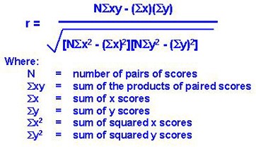
The formulae of Pearson Coefficient of correlation is as shown below
N
3.00
N∑xy
1,135,037,529.00
∑x∑y
1,125,065,350.00
N∑x^2)
8,272,006,539.00
∑x^2)
2,757,335,513.00
N∑y^2)
159,371,202.00
∑y^2)
53,123,734.00
Coefficient of correlation (r) = 1,135,037,529.00-1,125,065,350.00/ Square root of (8,272,006,539.00-2,757,335,513.00)( 159,371,202.00- 53,123,734.00)
After conducting Pearson coefficient of correlation, the result was a positive correlation of the variables. This means that when sales increase, the operating income increases too. This shows that we can predict the outcome of the year 2015.
Conclusion
From the project, it is evident that statistic can be used to predict outcome. Therefore, the research question has been addressed well. From the analysis, it has become evident that the use of statistic is faced with certain challenges. Firstly, reliability of some data sources is questionable. Additionally, the fact that data is not readily available is another challenge. There has also been an important observation that the choice of variables should be done properly to avoid confusion of the tests carried out. From the project, it has come out clearly that when there is positive correlation of variables, the movement of change in any of them is positive.
Inferential Statistics and Findings: Generating a Hypothesis
The aim of the paper is to generate a hypothesis with the use of research questions and two variables- dependent variable: sales/revenue and independent variable: interest rates. In addition, the paper uses a statistical technique for testing the hypothesis at 95% confidence interval while interpreting the results. XYZ Corporation is a US-based company that majors in home improvement and construction.
Moreover, the company operates in various big-box format stores across the United States. Nevertheless, XYZ Corporation wants to determine the effects of interest rates and sales on its future profitability, therefore, the company approached a research team that suggested the below research question.
Research question
Is there a relationship between federal (Feds) directed interest rate (ID) and sales /revenue (DV) on future profit of XYZ Corporation?
Hypothesis H0 = XYZ Corporation’s future profits are not determined by interest rates and sales/revenue H1 = XYZ Corporation’s future profits are determined by interest rates and sales/revenue
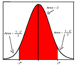
Hypothesis tests with a 95% confidence level
The veracity of the null hypothesis depends on data as well as the objective of significance tests to estimate the likelihood, hence the P-value, which underscores that the occurrence is an issue of chance. In this case, if the Pearson Correlation is less than 5% it means that the null hypothesis is rejected.
However, if the P-value is greater than 5% then it means the statistical test fails to reject the null hypothesis (Gupta, 2012). Data was indiscriminately selected from 382 observations with respect to interest rates and sales of XYZ Corporation.
Interpretationof the results and findings
Statistical analysis demonstrates that this is a normal distribution, with a mean of 10.97644 and standard deviation of 10.14628 for sales (Table 1). In this case, sales were observed between $0.00 and $89.00. Changes in the federal interest rates could help determine sales of XYZ Corporation.
In addition, the mean and standard deviation for interest rates were observed at 9.695538 and 7.836266 respectively (Table 2). High-interest rates are highly likely to inhibit any profit making from lack of sales. While low-interest rates by the federal government may lead to increased sales.
Again, it demonstrated a 95% confidence interval (sales:1.020716, interest rates: 0.789369) this implies that XYZ Corporation can be about 95 percent confident that sales and interest rates will lead to an increased future a profit. Because the confidence interval of sales corresponds to the value of alpha, which is 1 indicates that there is no significant correlation between sales and future profit of XYZ Corporation.
However, the results are empirically reliable. When it comes to interest rates the confidence interval is less than 1, statistically the test fails to refute the null hypothesis, an aspect that demonstrates statistical significance of the test (Monette, Sullivan & DeJong, 2011).
Gupta, S. K. (2012). The relevance of confidence interval and P-value in inferential. Indian Journal of Pharmacology. Retrieved on June 9, 2016, from statistics http://www.ncbi.nlm.nih.gov/pmc/articles/PMC3271529/
Monette, D. R., Sullivan, T. J., & DeJong, C. R. (2011). Applied Social Research: A Tool for the Human Services (8th ed.). Belmont, CA: Brooks/Cole.
Want help to write your Essay or Assignments? Click here
This report is an analysis of the data generated using SPSS and presented using charts and tables. The report firstly presents the results of selected descriptive statistical analyses. Subsequently, the report summarises the numerical results with descriptive statistics analysis tables or graphs, including the interpretation of these tables and graphs. The fourth section or the report is a presentation of the data regarding numerical results of the inferential statistics. This is followed by a discussion of the same, before a summative conclusion is presented in the last section.
Selected descriptive statistics
Descriptive statistics refers to the kinds of data that analysts and researchers use in presenting the characteristics of the sample used in a study. According to Kothari (2004), they are used in checking whether the variables that the researcher has chosen to use violate any assumptions that the researcher might have made, which might be consequential to the findings. Another important function of descriptive statistics used in this section is that they help to answer the core research questions.
In the present study, the descriptive statistics selected are for public use micro data area code (PUMA), house weight (WHTP), state code, (ST), numbering of persons (NP), rooms (RMS), bedrooms, (BDS), and household income (HINCP). The data retrieved was as presented in table 1 below
Table 1: PUMA, ST, BDS, RMS, mean, median, and standard deviation
RMS
BDS
ST
PUMA
N
Valid
4911
4911
4911
4911
Missing
0
0
0
0
Mean
4.87
2.61
15.00
248.05
Median
5.00
3.00
15.00
302.00
Std. Deviation
1.933
1.197
.000
81.573
Minimum
1
0
15
100
Maximum
9
5
15
307
Table 2: RMS, BDS, ST, and PUMA, frequency table
PUMA
Frequency
Percent
Valid Percent
Cumulative Percent
Valid
100
951
19.4
19.4
19.4
200
782
15.9
15.9
35.3
301
407
8.3
8.3
43.6
302
412
8.4
8.4
52.0
303
425
8.7
8.7
60.6
304
536
10.9
10.9
71.5
305
365
7.4
7.4
79.0
306
456
9.3
9.3
88.3
307
577
11.7
11.7
100.0
Total
4911
100.0
100.0
NP
Frequency
Percent
Valid Percent
Cumulative Percent
Valid
0
452
9.2
9.2
9.2
1
970
19.8
19.8
29.0
2
1491
30.4
30.4
59.3
3
711
14.5
14.5
73.8
4
619
12.6
12.6
86.4
5
318
6.5
6.5
92.9
6
161
3.3
3.3
96.2
7
94
1.9
1.9
98.1
8
30
.6
.6
98.7
9
20
.4
.4
99.1
10
18
.4
.4
99.5
11
7
.1
.1
99.6
12
7
.1
.1
99.7
13
5
.1
.1
99.8
15
1
.0
.0
99.9
16
2
.0
.0
99.9
17
1
.0
.0
99.9
19
2
.0
.0
100.0
20
2
.0
.0
100.0
Total
4911
100.0
100.0
RMS
Frequency
Percent
Valid Percent
Cumulative Percent
Valid
1
185
3.8
3.8
3.8
2
345
7.0
7.0
10.8
3
677
13.8
13.8
24.6
4
896
18.2
18.2
42.8
5
1110
22.6
22.6
65.4
6
768
15.6
15.6
81.1
7
438
8.9
8.9
90.0
8
234
4.8
4.8
94.7
9
258
5.3
5.3
100.0
Total
4911
100.0
100.0
BDS
Frequency
Percent
Valid Percent
Cumulative Percent
Valid
0
211
4.3
4.3
4.3
1
683
13.9
13.9
18.2
2
1208
24.6
24.6
42.8
3
1810
36.9
36.9
79.7
4
688
14.0
14.0
93.7
5
311
6.3
6.3
100.0
Total
4911
100.0
100.0
From the data in table 1 above, a number of observations are blatant and clear. The first is that the means of RMS, BDS, ST and PUMA are 4.87, 2.61, 15, and 248.05 respectively. For rooms, the number of rooms, the median score was 5, where the scores varied from 1 to 9. This means that the majority of respondents have about 5 rooms.
When it comes to the number of bedrooms, the median score was 3, whereas the mean was 2.61, this shows that the majority of respondents have 3 rooms. The state code was 15 for all respondents whereas the mean for public use of micro data area code was 248.05. The mean was 302, whereas the minimum and maximum scores were 100 and 307 respectively.
From table 2, a number of assertions can also be made, and the first is about PUMA. From the table, the evidence shows that for public use of micro data area code, 19.4% of the respondents scored category 100, which made it the highest selected category, whereas 15.9% of the respondents checked 200, making it the second most selected category. Comparatively, 301 was the least selected category at 8.7%.
Additionally, for number of bedrooms, a majority of the respondents said that they had three bedrooms in their houses, and this represented 3.9% of all responses, closely followed by those with two bedrooms at 24.6%. At the same time, the number of people living in houses with no bedrooms or five bedrooms was the least with a score of 4.3% and 6.3% respectively.
This data is in line with the data about rooms, which shows that 22% of respondents stay in a five-roomed apartment, followed by 18% and 15%, who stay in four and five roomed houses respectively. Because of the number of rooms and bedrooms in their houses, it is plausible to conclude that a majority of the respondents stay with other people or expect other people to visit often, which are why they have extra rooms in the house, as well as extra bedrooms in the house.
Additionally, from the data, it is obvious that a majority of the people are in the middle between the rich and the poor, as those who stay in studio apartments are as marginal as those who stay in luxury apartments that can contain at least five bedrooms. .
Selected inferential statistical analyses
Inferential statistics refer to the data analysis methods where the researcher or analyst uses a given set of data to determine whether there is a link between given variables being studied. By using inferential statistics, the researcher can tell whether the relationship that seems to exist between variables is a fact, or whether it is not a fact. According to Kothari (2004), a number of measures and techniques can be used to accomplish inferential statistics. The two types of inferential statistics used in this report are correlation and regression analyses.
Correlation was conducted using the Pearson correlation analysis. Pearson correlation analysis is employed to measure the linear relationship between two or more variables. The value of Pearson correlation ranges between -1 and +1, with -1 indicating negative correlation, 0 indicating no correlation and +1 indicating positive correlation between the variables. Besides, the closer the value is to +1, the stronger the relationship between the variables (Saunders, Lewis & Thornhill, 2007). For this study, the data is as shown below.
According to table 4-20, Sig. (2-tailed) =0.000, and all the four variables have a significant correlation at the 0.01 significant level. Pearson correlation between PUMA and NP is .110, whereas the relation between PUMA and BDS and RMS is .042 and .067 respectively. This shows that there is a weak but positive relationship between PUMA and all the independent variables, although the weakest relationship is that between PUMA and BDS.
Table 3: Correlations
PUMA
NP
BDS
RMS
PUMA
Pearson Correlation
1
.110(**)
.042(**)
.067(**)
Sig. (2-tailed)
.000
.003
.000
N
4911
4911
4911
4911
NP
Pearson Correlation
.110(**)
1
.447(**)
.396(**)
Sig. (2-tailed)
.000
.000
.000
N
4911
4911
4911
4911
BDS
Pearson Correlation
.042(**)
.447(**)
1
.878(**)
Sig. (2-tailed)
.003
.000
.000
N
4911
4911
4911
4911
RMS
Pearson Correlation
.067(**)
.396(**)
.878(**)
1
Sig. (2-tailed)
.000
.000
.000
N
4911
4911
4911
4911
** Correlation is significant at the 0.01 level (2-tailed).
Regression analysis helps estimate and investigate the association between variables. R Square is used to show the degree of relationship between the dependent and independent variables. R Square value ranges between 0 and 1, and the closer the value is to 1, the stronger the relationship between the variables further indicating the greater degree to which variation in independent variable explains the variation in dependent variable (Seber and Lee, 2012).
Based on the model summary table 4-21, R stand for the correlation coefficient and it depicts the association between dependent variable and independent variables. It is evident that a positive relationship exists between the dependent variable and independent variables as shown by R value (0.126).
However, the relationship is a very weak one. Besides, it can be seen that the variation in the three independent variables (RMS, BDS and NP) explain 1.6% variation of PUMA as represented by the value of R Square. Therefore, it means that other factors that are not studied on in this study contribute 98.4% of the PUMA programs. This means that the other factors are very important and thus need to be put into account in any effort to enhance PUMA. Additionally, this research therefore identifies the three independent variable studied on in this research as the non-critical determinants of PUMA boundaries.
Table 4: regression analysis results
Model Summary
Model
R
R Square
Adjusted R Square
Std. Error of the Estimate
1
.126(a)
.016
.015
80.945
a Predictors: (Constant), RMS, NP, BDS
Further, this research established through the analysis f variance that the significant value is 0.00, which is less than 0.01, therefore the model is statistically significant in foretelling how NP, RMS, and BDS can influence PUMA groupings. The F critical value at the 0.01 level of significant was 26.501. Given that F calculated is greater than the F critical value of 26.501, then it means that the overall model was significant (Seber and Lee, 2012).
ANOVA(b)
Model
Sum of Squares
df
Mean Square
F
Sig.
1
Regression
520911.120
3
173637.040
26.501
.000(a)
Residual
32151092.845
4907
6552.087
Total
32672003.965
4910
a Predictors: (Constant), RMS, NP, BDS
b Dependent Variable: PUMA
At the same time, the beta coefficients also gives significant inferential information. According to the regression coefficients presented in table 4-23, this research found that when all independent variables (the number of persons (NP), number of rooms (RMS), and the number of bedrooms (BDS)) are kept constant at zero, the level of public use micro data area code (PUMA) will be at 231.13. A 1% change in number of persons will lead to an 11.4% increase in PUMA, whereas a one percent change in BDS will lead to a 12.1% changes in PUMA.
Comparatively, a one percent change in RMS will lead to a 12.8 percent change in PUMA. This leads to the conclusion that of the three variavles, RMS leads to the largest impact in PUMA when the three independent variables are pitted together. Further the statistical significance of each independent variable was tested at the 0.01 level of significance of the p-values.
Coefficients(a)
Model
Unstandardized Coefficients
Standardized Coefficients
t
Sig.
B
Std. Error
Beta
1
(Constant)
231.130
3.161
73.128
.000
NP
4.700
.654
.114
7.181
.000
BDS
-8.222
2.068
-.121
-3.977
.000
RMS
5.384
1.248
.128
4.315
.000
a Dependent Variable: PUMA
In general form, it can be said that the equation used to determine the link between Public use microdata area code, numbering of persons, rooms and bedrooms is of the form:
Y = β0+ β1X1+ β2X2+ β3X3+ ε
From the equation, β0 is a constant, whereas β1 to β3 are coefficients of the independent variables. X1 X2 and X3 are the independent variables numbering of persons, rooms and bedrooms respectively, whereas epsilon ε is an error term. Additionally, the dependent variable Y in the equation represents public use microdata area code. Pegging the present discussion in the formula above, the model would be as follows.
Y = 231.130 + .114X1 – .121X2 +.128X3
This means that the public use micordata area code = 231.130 + (0.114 x numbering of persons) – (0.121 x rooms) +(0.128 x bedrooms).
References
Kothari, C. (2004). Research methodology, methods & techniques (2nd ed.).New Delhi: Wishwa Prakashan.
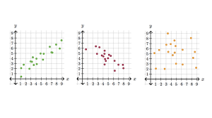
Scatterplots have been ranked as one of the oldest and most common techniques for projecting high dimensional data to 2-dimensional form. Generally, these projections are arranged in a grid structure to aid the user in remembering the dimensions linked with each projection. Scatterplots have proven to be quite useful in determining the relationship between two variables.
Scatterplots have been linked with a number of benefits. For instance, the plots have been cited as one of the most important technique for studying non-linear pattern. Krzywinski & Altman (2014) state that it is easy to plot the diagram. It is also useful in indicating the range of data flow, that is, the minimum and maximum value. Observation and reading of data in scatterplots is also straightforward.
Scatterplots are also important in studying large data quantities and make it easier to see the relationship between variables and their clustering effects. The use of scatterplots is an invaluable which is also useful in analyzing continuous data. However, this technique has a number of shortcomings such as being restricted generally to orthogonal views as well as challenges in projecting the relationship that exists in more two dimensions.
Question 2
When determining the appropriateness of the inferential statistical techniques, the researcher should first know if his/her data is arranged in a nested or crossed manner. If data is in a crossed manner, all study groups should have all intervention aspects. However, in a nested arrangement each study group will be subjected to a different variable. The correlation of variables can also be used in determining the appropriateness of a technique.
If the two variables have a linear or closely related association, the technique is said to be suitable. The number of assumptions that are employed when using a technique are also useful indicators. For instance, some techniques such as the t-test have several assumptions compared to the ANOVA technique, this implies that t-test has a large room for study errors unlike the ANOVA test.
Question 3
The Pearson product-moment correlation coefficient (PPMCC) is an analytical technique that is applied in indicating the strength of a linear association between two variables. This technique indicates a line of best fit through the data of two variables. It takes values ranging from +1 to -1 whereby a value of zero indicates that two variables of study do not have any association.
Values that are less than zero indicate that the two study variables have a negative association such that when one value increases the other one decreases. On the other hand, values that are greater than zero indicate that they have a positive association between them, that is, when there is an increase in one value, the other value increases as well. To determine whether the two variables have a linear relationship, they are fist plotted on a graph followed by a visual inspection of the shape of the graph.
A section of some scholars used to argue that PMCC can be used to indicate the gradient of a line. However, recent studies have dismissed this claim. For instance, Puth, Neuhäuser & Ruxton (2014) illustrate clearly that a coefficient of +1 does not mean that when one variable increases by one unit the other one increases by the same margin. A coefficient of +1 means that no variation exists between the plots and the line of best fit.
A number of assumptions must be put into consideration by analysts when they use the PPMCC. For instance, it is assumed that the outliers are either maintain at a minimum or removed completely. However, this is not the case in majority of studies. Another assumption is that the variables used should be distributed approximately normally and they must either be ratio or interval measurements.

 . Often, this parameter is the population mean
  , which is estimated through the sample mean